
Graphs — frequently used in the fields of transport, telecommunication, biology, sociology and others — allow, in the simplest cases, an exploration of data and their connectivity from a simple visual analysis. However, in most applications, for example in the classic case of the representation of social networks, the graphs obtained contain an immense quantity of nodes and connexions between them. When that’s the case, simple visual analyzes can quickly become complex. The use of machine learning on massive data graphs is a solution for numerous analytical and predictive approaches such as clustering for community detection, social link inference, vertex classification without a label, etc.
Deep learning is inspired by the functioning and architecture of brain systems: it uses artificial neural networks capable of solving complex problems with training. Deep learning seeks to learn through an algorithm composed of various layers of artificial neurons. The higher the number, the more the algorithm can handle with complex problems. In the context of large data volume processing, the use of deep learning and more specifically convolutional neural networks seems to be appropriate. Indeed, unlike multilayer perceptrons, convolutional neural networks limit the number of connections between neurons from one layer to another, which has the advantage of reducing the number of parameters to be learned.
Recent research is concerned with the application of convolutional neural networks to graphs. Convolutional neural networks are generally used for processing data defined in a Euclidean space (finite dimensional vector space) such as images structured on a regular grid formed by ordered pixels. However, graphs have no set structure or order allowing them to be processed in this way by convolutional neural networks.
A recent method called “Deep Graph Convolutional Neural Network” (DGCNN) proposed by M.Zhang et al. (2018) [1] exposes a new architecture of convolutional neural networks for graph processing.
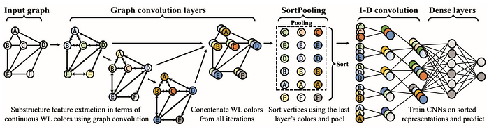
This new architecture proposes the addition of two steps (graph convolutions and Sortpooling) to allow graphs to be processed by traditional convolutional neural networks [1].
Graph convolution layers
Weisfeiler-Lehman Subtree kernel :
The extraction of information from the DGCNN method graphs is inspired by the Weisfeiler-Lehman subtree kernel method (WL)[2]. This method is a subroutine aimed at extracting features from sub-trees at several scales for graph classification. Its operation is determined as follows:

The basic idea of WL is to concatenate the color of a vertex with the colors of its neighbors at 1 jump thus contenance the signature WL of the vertex (b), then to sort the signature strings lexicographically to attribute new colors ©. Vertices with the same signature are given the same new color (d). The procedure is iterated until the colors converge or reach a maximum iteration h. In the end, vertices with the same converged color thus share the same structural role in the graph and are no longer distinguished. WL is used to check the isomorphism of graphs, because if two graphs are isomorphic, they will have the same set of WL colors at each iteration. The core of the WL subtree uses this idea to measure the similarity between two graphs G and G’: after iteration, the similarity is determined by the calculation of the kernel function (e)[2].
The DGCNN method differs from of WL. In fact, it doesn’t use the WL sub-tree method as such but uses a soft WL version. In this method, the kernel function isn’t calculated and the use of colors is not the same: the DGCNN method concatenates the colors obtained in the form of a tensor Zt (with t = 1, .., h) horizontally in a tensor Z1: h (h being the number of iteration / convolution performed) [1].
SortPooling
The major innovation of the DGCNN method is a new layer named SortPooling. SortPooling takes as input the characteristics of unordered vertices of a graph from the convolutions of graphs. Then, instead of summarizing the features of the vertices (causing a loss of information) as traditional pooling layers do, SortPooling classifies them in a consistent order and produces a sorted graph representation with a fixed size, so that traditional convolutional neural networks can read the vertices in a coherent order and be trained on this representation.
Therefore, the main function of the SortPooling layer is to sort feature descriptors, each representing a vertex, in a coherent order, before feeding them into convolutional and dense layers of a single dimension. For the classification of images, pixels are naturally arranged following their spatial order, whereas to classify text, the alphabetical order is used to sort the words. For graphs, the SortPooling layer classifies the vertices according to their structural role in the graph as established by the WL subtree kernel method.
Formally, the outputs of the convolutional layers of the Zt graph are used to sort the vertices. The layer of SortPooling takes as input a tensor Z1: h of size 𝑛 * Σ𝑐𝑡, where each line is a vertex feature descriptor and each column is a feature channel. The output of SortPooling is a tensor 𝑘 * Σ𝑐𝑡, where k is an integer to define. In the SortPooling layer, the input Z1: h is first sorted by line according to Zh.
More precisely, a coherent order is imposed on the vertices of the graphs, which makes it possible to form traditional neural networks on the representations of sorted graphs. The order of vertices based on Zh is calculated first by sorting the vertices using the last channel of Zh in descending order. Such an order is similar to the lexicographic order. The SortPooling layers acts as a bridge between graph convolution layers and traditional neural network layers by backpropagating loss gradients and thus integrating graph representation and learning into one end-to-end architecture [1].
DGCNN in practice
Detailed information for using the DGCNN algorithm is on the authors’ Git.
Non Input dataset
The input data of the DGCNN method must have a specific format. Several steps are needed in order to obtain the appropriately formatted data. The datasets tested by the authors (available on the platform of the University of Dortmund) are reference datasets suitable for graph kernel technics. Datasets can be described by several text files: firstly, the obligatory text files for the continuation of method where n = total number of nodes, m = total number of edges and N = number of graphs :
(1) _A.txt (m rows) fragmented adjacency matrix (diagonal block) for all graphs, each row corresponds to (row, column) resp. (node_id, node_id)
(2) _graph_indicator.txt (n rows) column vector of graph identifiers for all nodes of all graphs, the value in the i-th line is the graph_id of the node with node_id i
(3) _graph_labels.txt (N rows) class labels for all graphs in the dataset, the value in the i-th row is the graph class label with graph_id i
(4) _node_labels.txt (n rows) column vector of the node labels, the value in the i-th line is the node with node_id i
Then the optional text files:
(5) _edge_labels.txt (m lines) labels for the edges in _A.txt
(6) _edge_attributes.txt (m lines) attributes for the edges in _A.txt
(7) _node_attributes.txt (n rows) node attribute matrix, the comma separated values in the i-th row are the attribute vector of the node with node_id i
(8) _graph_attributes.txt (N rows) the regression values for all the charts in the dataset, the value in the i-th row is the graph attribute with graph_id i
The data contained in these files are only of numeric type: more precisely, the values can either be discrete or continuous. The data contained in these files are not directly usable by the DGCNN algorithm. The algorithm requires them to be transformed into a final single text file organized as follows:
N
n l
t m d
Where N is the number of graphs, n is the number of nodes per graph, l is the label of the graph, t is the label of the current node, m is the number of neighboring node of the current node (followed by the labels of each of these neighboring nodes) and finally d are the features of the current node (not mandatory). This transformation also includes generation of ten training samples and ten other test samples (each sample being a text file).
Launch of DGCNN algorithm
The DGCNN algorithm consists of several scripts. It requires the use of a machine with a GPU which is approximately forty times faster than the CPU (allowing rapid processing of matrix products and convolutions ). The Pytorch package is also needed for script execution, which is used to exploit the power of the GPU.
For each data set, it is possible to adjust the hyperparameters concerning the number of epochs, the number of batches per period, the size of the convolution filter, the learning rate, etc.
The execution of the algorithm is done from the next command where DATANAME precise which dataset is used:
./run_DGCNN.sh DATANAME
For each epoch, the algorithm displays the loss and accuracy of the training and the test phase.
Adaptability of DGCNN
Variations of graph structures
The datasets initially tested (PROTEINS and IMDB-M) pertain to the fields of biology and cinema. Each field of study has different graphs structures, it’s easy to imagine that graphs representing molecules and others representing movies characteristics would have very different structures.

In order to evaluate the DGCNN’s adaptability when faced with graphs containing datasets from different domains, we tested three new datasets coming from the platform of the University of Dortmund (AIDS, CUNEIFORM and MSRC_21).
If we take as an example the AIDS dataset (composed of 2 000 graphs each representing a chemical component), the goal consist in detecting the components with or without a particular sub-structure reflecting anti-HIV activity and classifying them into two distinct classes. According to the results from the previous table, the algorithm’s classification accuracy doesn’t seem to depend on the structure of the data. In other words, the algorithm seems to be applicable to graphs of various structures (except for the CUNEIFORM dataset which deals with the field of literature and history).
Others datasets formats
According to previous results, the DGCNN method seems to be adaptable to various types of data from numerous fields of study. To pursue this line of inquiry, we would like to test the method on a concrete case starting from a graph’s dataset contained in a graph-oriented database. These tested data do not have the required form to be processed by the DGCNN algorithm, so various transformations have to be performed (all details and code for transformation are available on this git page) :
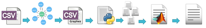
This on-going case study begins with the implementation of neighborhood crime data (CSV file) in the form of nodes and relationships in the Neo4j graph-oriented database, where each node represents a crime and is connected to adjacent neighborhood nodes. Cypher specific queries make it possible to organize the export of graph information to a csv file that has a particular shape and contains many superfluous characters.
The next step (Python script) allows to clean the data from the export Neo4j and partition the export into several text files in the data form proposed by the University of Dortmund. Finally, the information contained in these different text files will be assembled (Matlab script) in the final text file form used by the DGCNN algorithm. This last step also provides sample for training and test.
This method of transformation makes it possible to use data of different formats by converting them to the required format for DGCNN processing. The second part of the case study (in progress) will consist in running the DGCNN algorithm on this transformed data.
Conclusion
- The DGCNN algorithm makes it possible to establish a supervised classification on the data of graphs while preserving a maximum of information.
- According to tests performed on graphs dealing with various subjects, the DGCNN’s precision seems to be independent of the type of graph used.
- The required input data format of the DGCNN algorithm can be obtained after various transformations. It would be interesting to test the algorithm on data in other formats and from other domains.
[1] Zhang, Muhan et al. “An End-to-End Deep Learning Architecture for Graph Classification.” AAAI (2018).
[2] Shervashidze, Nino et al. “Weisfeiler-Lehman Graph Kernels.” Journal of Machine Learning Research 12 (2011): 2539–2561.
Future work orientation :
Hechtlinger, Yotam & Chakravarti, Purvasha & Qin, Jining. (2017). A Generalization of Convolutional Neural Networks to Graph-Structured Data.
Jian, Du & Zhang, Shanghang & Wu, Guanhang & Moura, Jose & Kar, Soummya. (2017). Topology adaptive graph convolutional networks.
Thanks to Luis Da Costa