This week, I took an interest in spatiotemporal data. There are several reasons why I have been looking into this subject. First, the City of Montreal makes available open data related to different spheres of activity: economy and business, education, health, society and culture. The sector that is of particular interest to me for Montreal is transportation.
CRIM has worked with spatiotemporal data to predict the response time of firefighters at the Service de sécurité incendie de Montréal. The article on this can be read on Medium. Given the experience gained during this project, it seemed logical to continue studying the subject. This new knowledge could eventually apply to resolving other mobility-related problems, such as travel in Montreal, thanks to the data collected by the MTL Trajet application or the cameras and detectors scattered around the Island of Montreal.
Spatiotemporal data also offers interesting potential from a local perspective for flood prevention in Quebec. In 2018, public security officials at the Ministère de la Sécurité publique unveiled a civil security plan of action in cases of flooding (the Quebec government release, in French, is found here) as a follow-up to the major spring floods of the previous year. Over five years, an envelope of more than $30M was provided to update the mapping of flood-prone areas on Quebec territory. In climatology, spatiotemporal data have become such an important tool that many data science projects are being developed to organize, analyze and interpret them.
Spatiotemporal data
Spatiotemporal data are collected in several fields: in climate science, to predict the onset of extreme weather events; in Earth science, to detect anomalous areas within marine environments; or in epidemiology, to study the spread of diseases. Other fields, such as neuroscience, environmental science, social media and traffic dynamics, also use such information in various ways.
But what is special about spatiotemporal data? They are characterized by spatial (distance, direction, position) and temporal (number of occurrences, changes in time, duration) attributes. In other words, they are data, or measurements, that change in time and space.
For example, for predicting meteorological events, the spatial representation is defined by a grid of the land area under study, and various parameters and atmospheric measurements characterize it. The temporal representation is then defined by the evolution of these parameters over time, which could allow, for instance, to design a prediction model of the evolution of hurricanes.
There is ample literature on the subject: the diversity of models, approaches and applications is practically countless. To begin with, I have limited myself to four articles of interest to give me an idea of how to manage and use spatiotemporal data.
The first paper presents an approach using a 3D convolutional neural network to learn spatiotemporal features. The second paper presents data mining applications using association rules in the context of hurricane analysis. The third deals with a learning model of hierarchical structures to predict the onset of extreme weather events. The fourth defines a spatiotemporal data mining model analyzing anomalous association structures in a marine environment. The following sections will summarize the essential and relevant ideas and concepts from each paper.
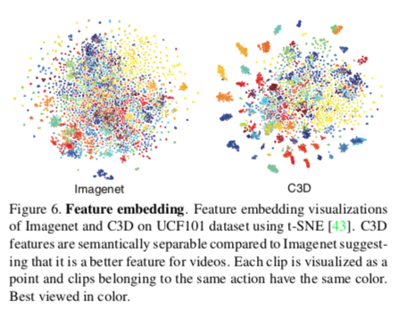
Learning Spatiotemporal Features with 3D Convolutional Networks
Tran, D., Bourdev, L., Fergus, R., Torresani, L., & Paluri, M. (2015, December). Learning spatiotemporal features with 3d convolutional networks. In Computer Vision (ICCV), 2015 IEEE International Conference on (pp. 4489–4497). IEEE.
Objective
Design of an approach for learning spatiotemporal features using a deep 3D convolutional neural network (3D ConvNets) trained on a large-scale supervised video dataset. The goal is to recognize different types of actions (101 actions) and objects (42 types) and to classify pairs of similar actions (432 actions) or individual scenes (14 scenes)
Summary

The idea behind 3D convolution operations is to preserve the temporal information of an input signal. Indeed, 2D convolutions applied on one or multiple images generate an image, thus a two-dimensional output. Only 3D convolutions preserve temporal information and generate a volumetric output. The same phenomenon is observed for pooling stages in 2D and 3D, respectively. Thus, using 3D convolutions to encapsulate the information related to objects, scenes and actions.
Method
Architecture
The basic architecture of the convolution kernel is a fixed receptive field of dimension {d x 3 x 3} where only the time dimension is modified for experimentation purposes. This limitation is due to the considerable training time that would result from numerous experiments. The notation for the dimensions of the video clips and kernels is as follows:
Video clip (c x l x h x w)
- c is the number of channels (different perspectives of an image, number of matrices defining it), l is the number of images, h is the height, w is the width
Kernel (d x k x k)
- d is the temporal dimension, k is the spatial dimension (identical height and width)
Basic parameters
Video clips are taken as input to subsequently establish their recognition or classification. The videos are 128 x 171 and are separated into clips of 16 images, with each frame divided into three channels (RGB). Several parameters can be modified to obtain the best possible results: number of convolution layers, pooling layers, fully connected layers, loss layers, filters per layer, and filling, stride, pooling size, batch size, learning rate and number of iterations.
Variations in parameters
Several parameter configurations are tested to optimize the encapsulation of the temporal information. In order to save time, only the temporal depth d of the kernel is modified. Two approaches are used:
Homogeneous temporal depth
- All convolution layers use kernels of identical temporal dimensions. Four configurations are tested, with depths of {1, 3, 5, 7}. For example, 1-1-1-1-1 for a five-layer convolutional architecture, where each kernel at each layer has a depth of 1.
Variable temporal depth
- The temporal depth of the kernel varies according to the convolution layer. Two configurations are tested, increasing and decreasing, respectively, with the following form: 3-3-5-5-7 and 7-5-5-3-3, for five-convolutional-layered architectures.
For homogeneous architectures, ones with a depth of three (3-3-3-3-3) provide the best results, and these perform better than the two heterogeneous architectures. It is also shown that increasing the spatial field does not improve the results. Therefore, the 3 x 3 x 3 architecture is retained when dimensioning the kernels.
Final architecture
Considering the previous experiments and given the computational and memory limits of the available hardware, the 3D convolutional neural network is presented as follows:

The 3D ConvNets contains eight convolution layers, each with, respectively {64, 128, 256, 256, 512, 512, 512} filters. These convolution layers allow images to be transformed and learn different features. Each kernel is of dimension {3 x 3 x 3} and has a stride of {1 x 1 x 1}.
The network contains five layers of max-pooling, an operation where only the maximum value of a region bounded by a kernel is retained to reduce the dimensionality of the input matrix. The kernels for the layers {pool2, pool3, pool4, pool5} are of dimension {2 x 2 x 2} and {1 x 2 x 2} for the pool1 layer. Each has a stride of {1 x 2 x 2}.
Two fully connected layers with 4096 output units follow convolution and pooling operations. They are necessary to classify the images from the high-level features provided by the convolution steps.
Results
The 3D ConvNets is tested on human action classification, action pair similarity, and scene and object recognition.
- The 3D ConvNets is better suited for spatiotemporal data than a 2D ConvNet, and is better at detecting information related to appearance and motion.
- A homogeneous {3 x 3 x 3} architecture of convolution kernels for each layer delivers the best performance.
- The features learned by the network, with a simple linear classifier, outperform or are comparable to those learned by current methods when the network is tested in four different application scenarios.
- The network is very user-friendly
- The 3D ConvNet initially focuses on appearance in the first few images, then tracks motion in the others.

- The features learned by the 3D ConvNets are compact and descriptive, as shown by the results following a dimensionality reduction using a Principal Component Analysis (PCA).
- The features show a good capacity for generalization.
Association Rule Data Mining Applications for Atlantic Tropical Cyclone Intensity Changes
Yang, R., Tang, J., & Sun, D. (2011). Association rule data mining applications for Atlantic tropical cyclone intensity changes. Weather and Forecasting, 26(3), 337–353.
Objective
Application of a data mining technique, Association Rule Data Mining, to analyze tropical cyclone (TC) intensity changes. The paper provides a user guide for this mining technique and a method for overcoming the low number of occurrences of some extracted weather conditions to improve the predictive capacity of the intensity of tropical storms.
Overview
The association rule mining technique provides a detailed picture of the dataset and allows the detection of relationships among multiple conditions that may be missed in a theoretical analysis. The study aims to apply this data mining technique automatically and without supervision. This mining provides “multiple to one” associations from various geophysical features describing intensifying, weakening or stable cyclones. The data mining results can shed light on the underlying physical mechanisms that influence changes in the intensity of tropical storms.
Data and methodology
Datasets
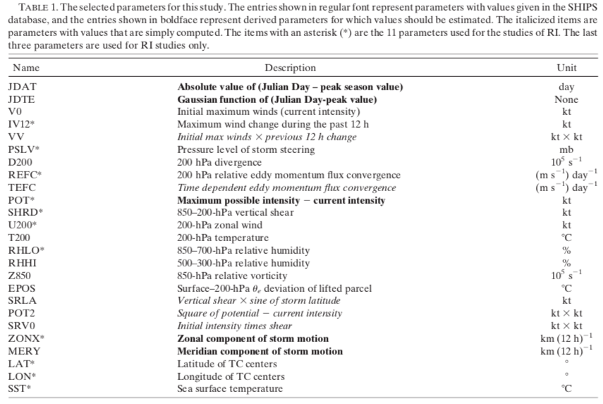
The HURDAT (NHC’s North Atlantic Hurricane Database) dataset was used to classify cyclone intensity and position. The SHIPS 2003 dataset obtained various parameters concerning tropical storms (21 features). The association rule implemented by Borgelt was subsequently applied to the dataset.
Definitions
An association rule takes on the following form: Z ← X, Y. In a business context, an example of a rule would be to say that a customer buying items X and Y is also likely to buy item Z. Items X and Y are called antecedents and Z is called the consequent.
In the context of the paper, the antecedents are the geophysical conditions of the CTs represented by an interval of values, and the consequent is a category of change in intensity (intensifying, weakening, etc.)
Three parameters are typically used for association rule exploration. Support estimates the probability P( { X, Y, Z } ), which is, for example, the frequency with which particular conditions for tropical storms (high/low wind speed, high/low pressure, etc.) occur in the dataset. Confidence estimates the probability P( Z | { X, Y } ), which is the frequency with which the particular tropical storm conditions caused a change in intensity Z. An association rule is strong if it has high support and confidence
The lift estimates the probability P( { X, Y, Z } ) / [ P( { X, Y } ) x P( Z ) ], that is, the ratio of the support computed above to that which would be expected if the conditions X and Y were independent. In other words, the lift gives the ratio of the actual probability that a set of items contains the antecedent and the consequent, divided by the product of the individual probabilities of the antecedent and the consequent. This is the ratio of confidence to expected confidence.
A lift of 1 would imply that the probability of occurrence of the antecedents and the consequent is independent. A lift greater than 1 would imply that the probability of occurrence of the antecedents and their consequent is dependent.
An example of an association rule will be explained hereafter to facilitate comprehension of the concept.
Stratification of cyclones and data pretreatment
Stratification
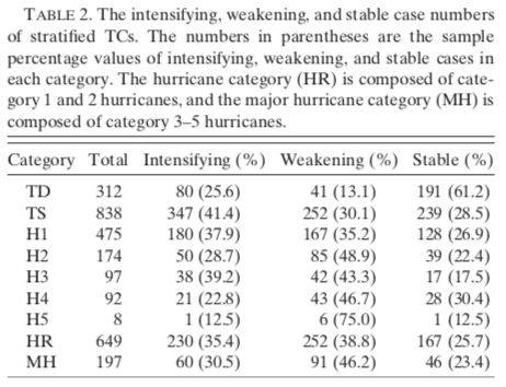
Since changes in the intensity of tropical cyclones depend on the initial intensity of these cyclones, the data set is divided into different groups. However, before stratifying the dataset, it is necessary to remove cyclones that do not have a complete set of parameters. The cyclones can then be grouped according to their initial intensity. These groups include:
- Tropical Depressions (TD)
- Tropical Storms (TS)
- Hurricanes (H1, H2, H3, H4, H5)
Two more categories are added, as class 5 hurricanes are infrequent. It is difficult to define rules with such a small sample, so a group containing hurricanes of class 1-2 and another containing classes 3-5 are introduced.
- Minor hurricane group (HR)
- Major hurricane group (MH)
To explore the combinations of factors influencing changes in intensity, cyclones are separated according to whether they intensify, weaken or remain stable (see Table 2).
Pretreatment
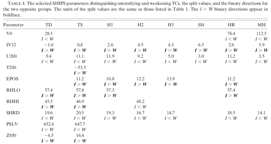
The association rule mining algorithm is initially designed to handle Boolean attribute datasets. In this case, the attributes of cyclones are numerical and continuous, so it is essential to transform them into binary conditions. Therefore, the spectrum of values is divided into two groups: low values and high values, according to a predefined threshold.
The threshold for each parameter is derived by taking the average of the respective averages of intensifying and weakening cyclones for each cyclone category. The relationship I > W (in bold) indicates that the average of the intensifying cases is considerably larger than that of the weakening cases and vice versa. This expression already gives an idea of the role of each parameter in the intensification or weakening of cyclones.
Association Rules

The rule mining association algorithm implemented by Borgelt was applied with the transformed binary parameters as priors to find combinations related to intensifying, weakening and stable cyclones. The abbreviations H and L represent high and low parameter values. For example, U200 = L in the TS case signifies that the 200-hPa zonal wind is less than or equal to 11.1 kt.
A priori, the parameters for controlling the weight of the rules are set to 33% for support and confidence and 100% for lift. Here is how to interpret an association rule.
A rule typically takes the following form:
INTENS ← U200 = L, SHRD = L, SRLA = L (38,7, 75,4, 138,9)
When all three conditions (U200 = L, SHRD = L, SRLA = L) are satisfied, a storm will intensify with 38.7% support, 57.4% confidence, and 138.6% lift.
In other words, for cyclones in the Tropical Storms (TS) category, 38.7% of the cases satisfy the conditions (U200 = L, SHRD = L, SRLA = L). Of these cyclones, 57.4% intensified, compared to the average sample of 41.4% intensifying. The lift represents the ratio of the confidence to the confidence of the average intensifying sample (57.4/41.4 = 138.6%) (57.4/41.4 = 138.6%)
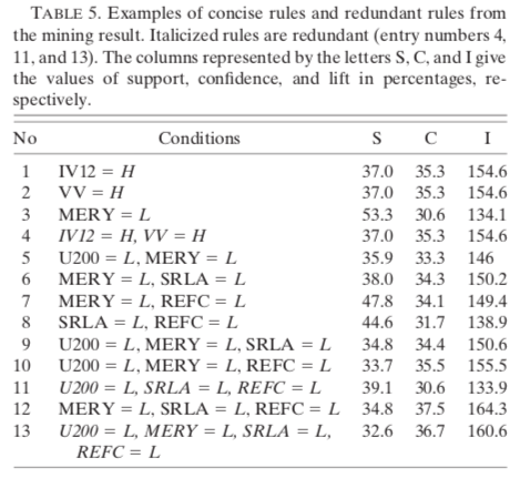
However, once the algorithm is applied, it is necessary to remove the redundant rules to consider only the concise rules. A rule is concise if it cannot be derived by a subset of priors from another rule with higher confidence. In other words, a concise rule contains the smallest number of priors. Any rule that contains the same antecedents and additional antecedents, but does not have a higher confidence than a concise rule, is redundant.
For example, rule 4 (see Table 5) is redundant because it has the same confidence as rules 1 and 2. Rule 11 is redundant because it contains a combination of conditions appearing in rule 8 and has a lower confidence than rule 8.
Intramural Binding
Some parameters cover the same physical process: for example, IV12 and VV quantify a cyclone’s past intensity change. Others are all associated with vertical shear: U200, SHRD, SRV0 and SRLA. When the values of one parameter can be used to predict the values of another, they are said to be intramurally bound.
Association hyper-edges were generated using the same association rule mining algorithm to reveal these links. The results showed a perfect link between IV12 and VV for all categories except the MH group and a strong link between U200, SHRD, SRV0 and SRLA. This is another interesting result of this data mining technique.
Results
This study showed that the rule mining association can be used successfully in geoscience.
- Ease of interpretation of results.
- Combinations of parameters were found, allowing to group conditions favouring the intensification or weakening of cyclones.
- A faster northward movement of cyclones favours the intensification of tropical storms but not hurricanes.
- Intensifying tropical storms are more strongly associated with high convergence in the upper atmosphere (200-hPa relative eddy momentum flux convergence) than weakening ones while intensifying hurricanes are more strongly associated with lower convergence values.
- The combinations of conditions identified provide higher probabilities of intensification/weakening than those based on a single condition (typical of traditional statistical studies).
- This study will lead to improved cyclone intensity prediction (TC).
A Hierarchical Pattern Learning Framework for Forecasting Extreme Weather Events
Wang, D., & Ding, W. (2015, November). A hierarchical pattern learning framework for forecasting extreme weather events. In Data Mining (ICDM), 2015 IEEE International Conference on (pp. 1021–1026). IEEE.
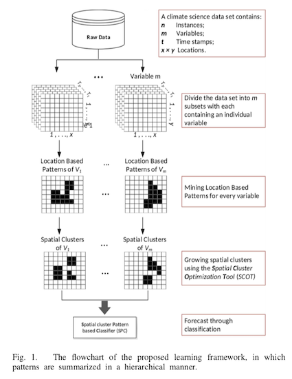
Objective
Design a model to discover structures (patterns) within a spatiotemporal system to predict extreme weather events. The structures are discovered hierarchically, i.e. at each level of learning, new contextual features are learned and used by the next level. Several difficulties must be overcome to deal with such a system:
- The massive size of the feature space.
- The presence of complex structures within the spatiotemporal system.
- The strict requirements for the interpretability of the model: We want to understand, not just predict.
Summary
- Summarize the temporal evolution of individual variables. At each position, the temporal changes of a parameter are generalized into a single feature.
- Summarize spatial relationships to assemble singular features into groupings.
- Summarize intervariable relationships to predict extreme events.
Definitions
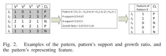
Features and feature sets
A feature is a tuple {L, T, V}. V is a domain variable. L indicates the position (x, y), and T indicates the sampling time.
A feature set is a variable sampled over a time range. A variable sampled from a time T1 to T4 will be considered a feature set of the form {V1, V2, V3, V4}.
Patterns and location-based patterns
A pattern X is a set of feature-value pairs corresponding to a set of features. It is a rule constructed from possible feature values for a certain set. For example, X = {< V1, 1 >, < V2, 0 to 4 >, < V3, 1 or 2 >, < V1, 3 >}.
A location-based pattern has the form of a tuple {X, L}. X represents a pattern, and L contains the spatial information of the pattern.
Support and growth ratio
A pattern X is supported by an instance I from a dataset D if the feature values of the instance I conform to the rule specified by the pattern X. The support of a pattern X is the number of instances I from a dataset D that support it, divided by the total number of instances I in D. In other words, the support is an indication of how often a pattern X appears in a data set D.
If we divide D into two partitions {Dp, Dn}, the growth ratio of a pattern X is the ratio of the support of X in the partition Dp to the support of X in the partition Dn.
Feature of a pattern
The feature of a pattern X is a binary variable indicating if the pattern is present or not in an instance I.
Method
Learning location-based patterns
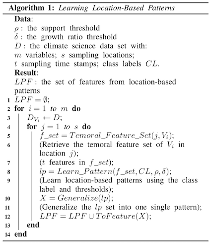
The first algorithm based on contrast pattern mining is used to learn location-based patterns. To begin with, the dataset is partitioned into m subsets, each containing one variable. The location-based patterns are then learned (line 3). Pattern sets are generated separately for each subset and each position within them (lines 4-8). At each position, the learned pattern sets are generalized into a representative singular pattern, which is then transformed (line 9). For example, for a position (x, y), the set of patterns {p1, p2, …} of a variable V represents the set of revealing temporal changes that occurred more frequently than others in a dataset partition.
Forming spatial groupings
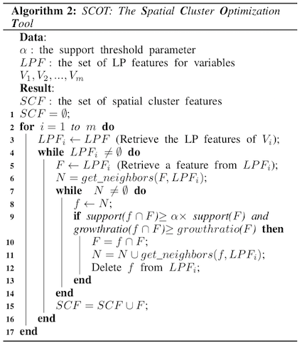
For this second algorithm, the spatial regularities of the system are generalized by expanding the previously learned location-based patterns into spatial clusters. Each variable is treated separately (lines 2-3). For a variable V1, a feature F is retrieved from its set of location-based patterns (line 5), and a set N containing all spatial neighbours of F is created (line 6). For all features f in N, two conditions are tested by linking with the support and growth ratio of the joined structure f ∩ F (line 9). If the conditions are satisfied, the patterns f and F are combined into a new pattern, and the neighbour set is updated by adding the neighbours of f in N (lines 10-11).
Provide for by classification
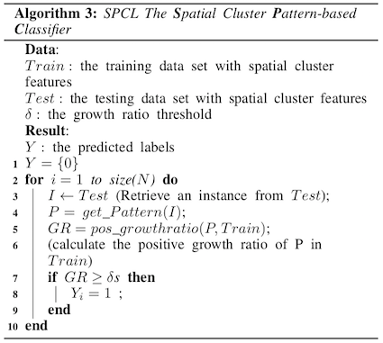
The final algorithm examines the interactions between variables by developing a Spatial cluster Pattern-based Classifier (SPC), an instance-based learning algorithm. An instance is classified by analyzing its patterns within spatial clusters (lines 3-4) and calculating the pattern growth ratio (lines 5-9). The instance is positively classified if it is higher than the predefined threshold.
Results
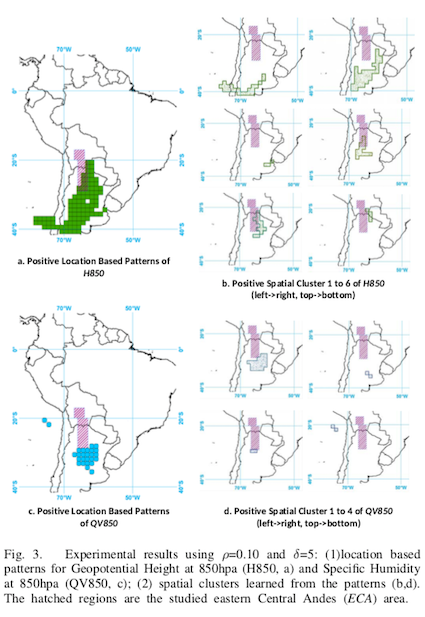
- The patterns learned from the approach in this paper are consistent with knowledge from studies in the same field.
- Increasing the support thresholds and growth ratio increased the F1 value.
- Predicting by using spatial clustering features (SCFs) yielded better results than simply using location-based pattern features (LPFs).
- SCFs reduce the risk of overfitting and provide a better growth ratio to the benefit of support.
A spatiotemporal mining framework for abnormal association patterns in marine environments with a time series of remote sensing images
Xue, C., Song, W., Qin, L., Dong, Q., & Wen, X. (2015). A spatiotemporal mining framework for abnormal association patterns in marine environments with a time series of remote sensing images. International Journal of Applied Earth Observation and Geoinformation, 38, 105–114.
Objectives
Design a spatiotemporal data mining framework for marine association structures using multiple remote sensing images. The goal is to detect anomalous events based on pixel- and object-level models.
Difficulties
Considering the massive size of the feature space, as each pixel has its own spatiotemporal association pattern, finding an efficient way to discover marine spatiotemporal associations on a pixel-by-pixel basis is essential. The second problem is that these pixels must also be grouped to form analyzable objects.
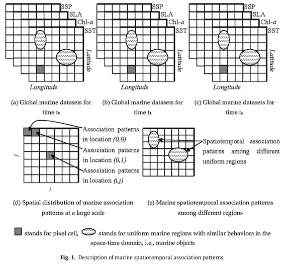
Two catalogues of association patterns are thus generated: in the same region (pixel, singular cell) and between different regions (object, grouping of pixels).
The spatial relationship of the association patterns in the first catalogue is simply the spatial positioning of the pixels. Despite the small contribution of these patterns to spatial relationships, the use of pixels alone is more suited to representing large-scale spatiotemporal association patterns. In the context of this study, this catalogue allows the analysis of the ocean as a whole.
For the second catalogue, the association patterns between regions with uniform marine properties (marine objects) provide more information on spatial relationships: spatial positioning, distance, direction and topology. This one will focus on specific marine regions compared to the first catalogue. The two catalogues are thus complementary in the search for spatiotemporal association patterns.
Summary
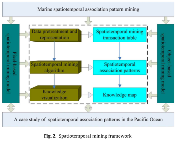
- Pretreatment and representation of data by a transaction table.
- Spatiotemporal data mining algorithm to generate association patterns.
- Knowledge visualization.
Method
Data pretreatment and representation
Eliminating periodic variability
Marine parameters are subject to seasonal variations: it is, therefore essential to remove this component to normalize the data before identifying abnormal events. To do this, the z-score, calculated monthly, is used. It indicates how many standard deviations an environmental parameter is from the mean and standardizes the value of this parameter accordingly.
Extracting anomalous objects
Regions sensitive to climate change are identified as anomalous regions and represented as objects in the context of this study. The ENSO (El Niño-Southern Oscillation) signal represents global climate variability, and the parameters influenced by this signal are identified. To do so, it is necessary to analyze whether the time component of a given physical factor is the same as that of ENSO (4-7 years) but also its spatial pattern. Subsequently, these regions sensitive to climate change and having the same associated spatial pattern are grouped as anomalous objects.
Discretizing marine parameters
Discretization consists in transforming marine parameters in real-number format into categories. The variability of the marine environment generally is Gaussian distributed. Consequently, the parameters are discretized into five classes, from -2 to +2 (severe negative change, weak negative change, no change, weak positive change, and severe positive change).
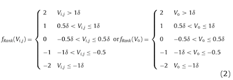
Where P(i,j) and O are, respectively, pixel position and instances of anomalous objects, Vi,j and fRank(Vi,j) are the raw value and class of a pixel, Vo and fRank(Vo) are the raw value and class of an anomalous object, 𝛿 and 𝛿o are the standard deviation of a time series of a pixel and an anomalous object.
Generating transaction tables
An exploration table is generated for analysis at each level of granularity: pixels and objects. The first model can explore spatiotemporal association patterns among marine environmental parameters within pixels.
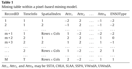
The second model allows us to discover the spatiotemporal association patterns between marine regions.

Spatiotemporal data mining algorithm
This algorithm is based on mutual information, i.e. the amount of information one item provides about another. The items are represented by the environmental parameters and the ENSO index (tables 1 and 2). The ENSO index is used to categorize the marine parameters according to the degree of influence of La Niña (-2) and El Niño (+2) on their evolution.
Association pattern mining algorithms find rules that define relationships between items in two steps. First, they discover frequent item patterns from the transaction tables using minimal support. Second, they generalize the association rule from a predefined confidence level. Only related items, rather than the complete set, are involved in the search for frequent items.
Extracting related items
Items are considered related or not based on their normalized mutual information. The mathematical approach will be set aside for ease of reading. Related items are extracted to provide candidates for the set of frequent items, which will be used to find association patterns. Not all related items are retained to be frequent; to do so, they must reach a certain relationship threshold. The frequent item set contains all the item patterns that appear frequently enough, according to a threshold, in the data set.
Generating association pattern trees
A direct association pattern tree represents the association patterns of two or more marine environmental parameters, thus providing a foundation for implementing a space-time exploration algorithm. A recursive method is applied to build this tree.

Discovering the rules of association
Generating association rules allows the discovery of frequent items originating from direct association pattern trees. To achieve this, transaction tables and direct association pattern trees are browsed using a recursive exploration algorithm. Specific evaluation indices are used to generalize strong association rules: support, confidence, lift and interest factors.
Visualizing spatiotemporal association patterns
Spatiotemporal association structures are represented as follows:

Where AttrN is a marine environmental parameter of a pixel or object, q is the quantitative level (-2 to +2) of this parameter, t is the time of occurrence of the attribute Attr1, {t1, t2 and tn} are the time differences from t when the other attributes occur, s%, c% and l% are the evaluation indicators used to identify revealing association patterns.
Although the association structures between objects and pixels are represented similarly, their spatial relationships differ. The spatial relationships between marine objects are implicit; topology, distance, and direction are all obtained from the objects. Spatial relationships between pixels are not as implicit; each pixel may have multiple spatiotemporal association patterns between two or more attributes.
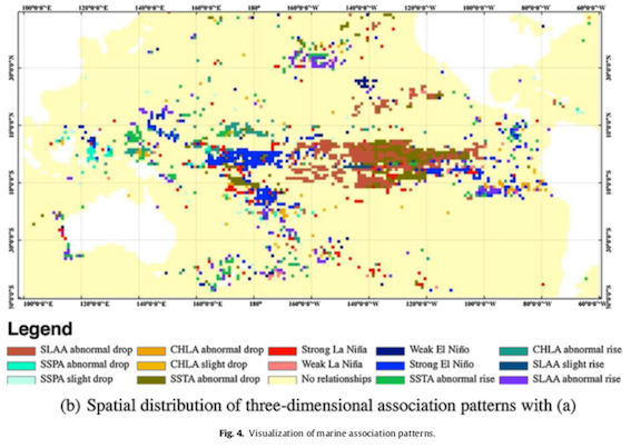
The spatiotemporal association patterns are represented on the following thematic maps. Note that the white regions define the different continents and the coloured regions the different association patterns in the Pacific Ocean. Map (a) shows the distribution of two-dimensional patterns, and (b) the distribution of three-dimensional patterns, as demonstrated by the association pattern tree.
For example, in Figure (a), we can see that when La Niña is strong, the ocean surface temperature (SSTA) drops drastically in the blue region.

Results
- The data mining algorithm based on mutual information is superior to the traditional Apriori algorithm in cases where more parameters and classes are used during discretization.
- Two proposed strategies: one model at pixel level and the other at object level. The two complement each other: the first explores large-scale marine features, and the second focuses on specific regions.
- Many problems were solved: extraction of associated items (attributes or objects), construction of direct association pattern trees, design of the exploration algorithm, optimal support threshold and innovative visualization of association patterns.
- Compared to traditional spatiotemporal analyses, the information obtained from this exploration framework is much more detailed and precise in space and time.
- This framework allows for a better understanding of the variation of marine parameters in different areas: how, when and where specific parameters drive the variation of other parameters or respond to the variation of others.


